Generate Handwritten Digits with GAN
Abstract: This tutorial introduces GANs by example. After showing it many real photos of handwritten digits, we will train a generative adversarial network (GAN) to generate new handwritten digits. Most of the code here comes from the gan implementation in examples\basic_tutorials\mnist_gan.py, and this document will explain that implementation in detail and elucidate the model's working and reasoning. But don't worry, prior knowledge of GANs is not required, but it may take a novice some time to infer what is actually happening behind the scenes.
Generative Adversarial Networks
What is a GAN?
GANs are a framework for teaching DL models to capture the training data distribution so we can generate new data from that same distribution. GANs were invented by Ian Goodfellow in 2014 and first described in the paper Generative Adversarial Nets. They are made up of two different models: the generator and the discriminator. The generator's job is to generate "fake" images that look like the training images. The discriminator's job is to look at an image and classify it as either being a real training image or a fake image from the generator. During training, the generator is constantly trying to outsmart the discriminator by generating better and better fakes, while the discriminator is working to become a better detective and correctly classify real and fake images. The equilibrium point of the game is when the generator is generating fakes that look indistinguishable from the real training images, while the discriminator is always guessing that the generator output is fake with 50% confidence.
Now let's define some symbols that we'll use throughout the tutorial. Let x be data representing an image. D(x) is the discriminator network which outputs the (scalar) probability that x came from training data rather than the generator. Here, since we are dealing with images, D(x)'s input is an image of size CHW with 3x64x64. Intuitively, when x comes from training data, D(x) should be high, and when x comes from the generator, D(x) should be low. D(x) can also be thought of as a traditional binary classifier.
For the generator's representation, let z be a latent space vector sampled from a standard normal distribution. G(z) represents the generator function which maps the latent vector z to data-space. The goal of G is to estimate the distribution that the training data comes from (p_data) so it can generate fake samples from that estimated distribution (p_g).
Because D(G(z)) is the probability (scalar) that the output of the generator G is a real image, log(D(G(z))) is the log-likelihood that G will output a real image, under the assumption that D is correct. Intuitively, this objective should cause G to output images that look as real as possible to D, so that D will output high probabilities for its inputs.
 From the paper, the GAN loss function is given by: From a theoretical perspective, the solution to this minimax game is where p_g = p_data, and the discriminator guesses randomly if the inputs are real or fake. However, the convergence theory of GANs is still being actively researched and in practice GANs do not always converge to this point.
1. Environment Configuration
This tutorial is based on TensorLayerX 0.5.6, if your environment is not this version, please refer to the official website installation.
TensorlayerX currently supports TensorFlow, Pytorch, PaddlePaddle, MindSpore as the computing backend, and the method of specifying the computing backend is also very simple, just set the environment variable
import os
os.environ['TL_BACKEND'] = 'paddle'
# os.environ['TL_BACKEND'] = 'tensorflow'
# os.environ['TL_BACKEND'] = 'mindspore'
# os.environ['TL_BACKEND'] = 'torch'
Import the required modules
import time
import numpy as np
import tensorlayerx as tlx
from tensorlayerx.nn import Module, Linear
from tensorlayerx.dataflow import Dataset
from tensorlayerx.model import TrainOneStep
2. Load Dataset
This case will use the API provided by TensorLayerX to download the dataset and prepare the data iterator for the subsequent training task.
The MNIST handwritten digit recognition dataset consists of 60000 black and white pictures of size 28 * 28. These pictures are divided into 10 categories, each corresponding to the numbers 0-9, and a model will be trained to correctly classify the pictures.
# prepare cifar10 data
X_train, y_train, X_val, y_val, X_test, y_test = tlx.files.load_mnist_dataset(shape=(-1, 784))
class MNISTDataset(Dataset):
def __init__(self, data=X_train, label=y_train):
self.data = data
self.label = label
def __getitem__(self, index):
data = self.data[index].astype('float32')
label = self.label[index].astype('int64')
return data, label
def __len__(self):
return len(self.data)
# prepare dataset and dataloader
train_dataset = MNISTDataset(data=X_train, label=y_train)
batch_size = 128
train_loader = tlx.dataflow.DataLoader(train_dataset, batch_size=batch_size, shuffle=True)
3. Build Network
Generator
Next, use TensorLayerX to define a neural network with three fully connected layers (Linear) and the first two layers use the relu activation function, and the last layer uses the Tanh activation function with a value range of -1~1 as the activation function of the neural network in the GAN as the generator network G, which maps a random noise vector of shape (1,100) through the fully connected layer to a vector of dimension 28*28=784, which is equivalent to generating a 28*28 handwritten picture.
class Generator(Module):
def __init__(self):
super(generator, self).__init__()
self.g_fc1 = Linear(out_features=256, in_features=100, act=tlx.nn.ReLU)
self.g_fc2 = Linear(out_features=256, in_features=256, act=tlx.nn.ReLU)
self.g_fc3 = Linear(out_features=784, in_features=256, act=tlx.nn.Tanh)
def forward(self, x):
out = self.g_fc1(x)
out = self.g_fc2(out)
out = self.g_fc3(out)
return out
Discriminator
Next, use TensorLayerX to define a neural network with three fully connected layers (Linear) and the first two layers use the relu activation function, and the last layer uses the Sigmoid activation function with a value range of 0~1 as the activation function of the neural network in the GAN as the discriminator network D, which accepts a vector of shape (1,784) from the generator network G or real handwritten pictures, which is folded into a vector by the fully connected layer and mapped to a vector of shape (1,1) with a value range of 0~1, corresponding to the two classification of real/fake.
class Discriminator(Module):
def __init__(self):
super(discriminator, self).__init__()
self.d_fc1 = Linear(out_features=256, in_features=784, act=tlx.LeakyReLU)
self.d_fc2 = Linear(out_features=256, in_features=256, act=tlx.LeakyReLU)
self.d_fc3 = Linear(out_features=1, in_features=256, act=tlx.Sigmoid)
def forward(self, x):
out = self.d_fc1(x)
out = self.d_fc2(out)
out = self.d_fc3(out)
return out
Print the model structure
Generator<
(g_fc1): Linear(out_features=256, ReLU, in_features='100', name='linear_1')
(g_fc2): Linear(out_features=256, ReLU, in_features='256', name='linear_2')
(g_fc3): Linear(out_features=784, Tanh, in_features='256', name='linear_3')
>
Discriminator<
(d_fc1): Linear(out_features=256, LeakyReLU, in_features='784', name='linear_4')
(d_fc2): Linear(out_features=256, LeakyReLU, in_features='256', name='linear_5')
(d_fc3): Linear(out_features=1, Sigmoid, in_features='256', name='linear_6')
>
4. Model Training & Prediction
Next, since the training process of the generator G and discriminator D two networks is mutually dependent, we need to wrap the calculation process of the loss function into a Module object.
class WithLossG(Module):
def __init__(self, G, D, loss_fn):
super(WithLossG, self).__init__()
self.g_net = G
self.d_net = D
self.loss_fn = loss_fn
def forward(self, g_data, label):
fake_image = self.g_net(g_data)
logits_fake = self.d_net(fake_image)
valid = tlx.convert_to_tensor(np.ones(logits_fake.shape), dtype=tlx.float32)
loss = self.loss_fn(logits_fake, valid)
return loss
class WithLossD(Module):
def __init__(self, G, D, loss_fn):
super(WithLossD, self).__init__()
self.g_net = G
self.d_net = D
self.loss_fn = loss_fn
def forward(self, real_data, g_data):
logits_real = self.d_net(real_data)
fake_image = self.g_net(g_data)
logits_fake = self.d_net(fake_image)
valid = tlx.convert_to_tensor(np.ones(logits_real.shape), dtype=tlx.float32)
fake = tlx.convert_to_tensor(np.zeros(logits_fake.shape), dtype=tlx.float32)
loss = self.loss_fn(logits_real, valid) + self.loss_fn(logits_fake, fake)
return loss
Then we use the TrainOneStep single-step interface to start the training of the model, which will:
Use the tlx.optimizers.Adam optimizer to optimize the G and D networks separately.
Use tlx.losses.mean_squared_error to calculate the loss value.
Use tensorlayerx.dataflow.DataLoader to load data and build batches.
Use tlx.model.TrainOneStep single-step training interface to build the model for training
loss_fn = tlx.losses.mean_squared_error
optimizer_g = tlx.optimizers.Adam(lr=3e-4, beta_1=0.5, beta_2=0.999)
optimizer_d = tlx.optimizers.Adam(lr=3e-4)
g_weights = G.trainable_weights
d_weights = D.trainable_weights
net_with_loss_G = WithLossG(G, D, loss_fn)
net_with_loss_D = WithLossD(G, D, loss_fn)
train_one_step_g = TrainOneStep(net_with_loss_G, optimizer_g, g_weights)
train_one_step_d = TrainOneStep(net_with_loss_D, optimizer_d, d_weights)
After that, we write a loop to load data from the dataset and train the train_one_step_g and train_one_step_d two networks
for epoch in range(n_epoch):
d_loss, g_loss = 0.0, 0.0
n_iter = 0
start_time = time.time()
for data, label in train_loader:
noise = tlx.convert_to_tensor(np.random.random(size=(batch_size, 100)), dtype=tlx.float32)
_loss_d = train_one_step_d(data, noise)
_loss_g = train_one_step_g(noise, label)
d_loss += _loss_d
g_loss += _loss_g
n_iter += 1
print("Epoch {} of {} took {}".format(epoch + 1, n_epoch, time.time() - start_time))
print(" d loss: {}".format(d_loss / n_iter))
print(" g loss: {}".format(g_loss / n_iter))
fake_image = G(tlx.convert_to_tensor(np.random.random(size=(36, 100)), dtype=tlx.float32))
plot_fake_image(fake_image, 36)
Epoch 1 of 50 took 1.3067221641540527
d loss: 0.5520201059612068
g loss: 0.19243632538898572
...
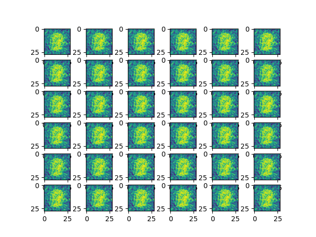
Image generated by GAN at the beginning:
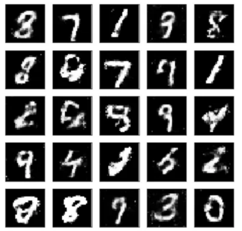
Final result:
The End
From the above example, we can see that using a simple GAN neural network on the MNIST dataset, we can generate realistic handwritten digit images with TensorLayerX. You can also achieve better results by adjusting the network structure and parameters.